Live Sources, Sound Cards and Tooling

Playing a converted file is the easy case: the whole signal exists before anything starts, nothing can run late, and if the result is wrong the file can be remade. Driving the kit from something happening now — a camera, a screen, a running program — is a different engineering problem, and most of its difficulty has nothing to do with television. It has to do with never letting an audio buffer run dry.

This volume covers the live case, the second tooling package in the hobby, the practicalities of using a modern computer’s sound card as a television transmitter, and what a builder writing their own encoder needs to know before writing it.

5.1 nbtv-design-tools

The second body of software worth knowing about is a SourceForge project called NBTV Design Tools, maintained by a developer identified there as vincent95 and registered on 18 May 2017. Its own summary describes it as “SW Tools + HW design example for Mechanical Narrow Band TV”, and more usefully: a set of software tools to create an NBTV video source, with audio and optionally with colour, on an ordinary two-channel PC audio output — plus a documented hardware design example.

What the project page and file listing establish:

Table 1 — What the project page and file listing establish

Release	Date listed	Size
nbtv-tools-and-doc-V1-0.zip	18 May 2017	5.0 MB
nbtv-tools-and-doc-V1-1.zip	19 May 2017	8.2 MB
nbtv-tools-and-doc-V1-2.zip	23 May 2017	29.6 MB
nbtv-tools-and-doc-V1-3.zip	8 September 2017	21.0 MB
nbtv-tools-and-doc-V1-4.zip	23 May 2019	36.6 MB
readme.txt	23 May 2019	566 bytes

The V1.4 release notes list corrections to the documentation per errata raised against 1.3, a new utility for creating compact 8-bit NBTV wave files (without sound), an Arduino-Player companion project folder, and a re-edited test file. The documentation lives inside the archive as nbtv-design-and-tools.pdf, and the project’s own readme directs users to it for everything. The project is listed for Linux and Windows, written in C and assembly, with a console interface, and aimed at advanced users.

Two honest notes. There is a date discrepancy worth flagging: the project summary gives version 1.4 as 12 May 2020 while the file listing dates the same archive 23 May 2019. Nothing important turns on it, but a reader chasing the newest release should not be surprised by two dates for one file.

And more significantly: the archive itself could not be opened for this volume. SourceForge refuses automated clients on every download path — the direct mirror URLs and its own canonical /files/<name>/download link all returned HTTP 403, with or without a referring page. No attempt was made to work around that. Everything above is therefore drawn from the project page, the file listing and the release notes, and the per-tool detail that would come from reading nbtv-design-and-tools.pdf is simply not in this dive. It is recorded as an open item in Vol 8: the package is a manual download away for anyone using a browser, and is worth reading before writing an encoder from scratch, particularly for its hardware design example and its Arduino player.

The relationship between the two packages is straightforward and they do not compete. video2nbtv (Vol 4) converts existing video into a wave file, on Windows, through a graphical interface. nbtv-design-tools generates NBTV video sources on a PC audio output, cross-platform, from a console — the tool for someone building a pipeline rather than converting a clip.

5.2 Live Versus Pre-Rendered: Where the Time Goes

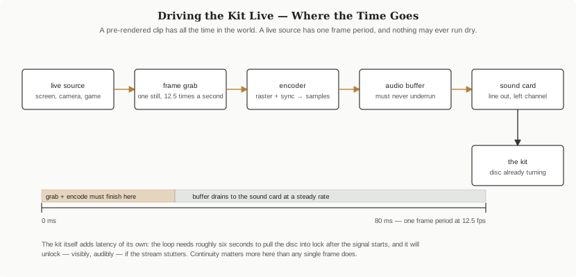
At 12.5 frames per second, one frame lasts 80 milliseconds. That sounds generous, and for the encoding arithmetic it is. The constraint is not per-frame compute; it is continuity.

Recall from Vol 2 how the kit acquires lock: the disc twitches, spins up as sync pulses arrive, makes a characteristic grinding noise approaching lock, and settles after a mean of roughly six seconds, with a worst case a little over twelve. That is the cost of acquiring lock — and it is paid again every time lock is lost. A stream that stutters for a few hundred milliseconds does not produce a few hundred milliseconds of glitch; it produces a lost lock followed by several seconds of rolling picture while the loop re-acquires.

This inverts the usual priorities of a real-time media pipeline. A dropped frame that is concealed by repeating the previous one costs almost nothing here. A gap in the audio output costs seconds. The design rule follows directly:

The sound card’s buffer must never underrun, even at the cost of showing stale pictures. Always have something to send. If the frame grabber is late, re-send the last frame. If the encoder is late, emit black with correct sync. Silence — or worse, a buffer gap — is the one output that must never occur.

5.3 Sample-Rate Arithmetic, and a Trap

Anyone writing an encoder meets this immediately, and it is worth getting right on paper first.

At the standard 44.1 kHz sample rate, one frame of 32 lines at 12.5 frames per second occupies:

44,100 ÷ 12.5 = 3,528 samples per frame, exactly.

That is a clean number, and it means a frame-length buffer can be built with no accumulating error. But divide it by the line count:

3,528 ÷ 32 = 110.25 samples per line.

Not an integer. Line boundaries do not land on sample boundaries. An encoder that emits a whole number of samples per line — 110, say — will produce a frame 8 samples short, and that error accumulates into a picture that drifts steadily sideways and eventually loses framing altogether. The error only cancels every four lines (441 samples per four lines, exactly).

Two workable approaches: carry a fractional accumulator so that lines alternate between 110 and 111 samples in the correct pattern, or — simpler and more robust — generate each frame as one 3,528-sample block and compute every sample’s position from its offset within the frame rather than from a per-line counter. The second approach makes the arithmetic error impossible by construction, which is worth more than the few cycles it costs.

Sync pulse width from Vol 3 is 0.1 to 0.25 milliseconds, which at 44.1 kHz is roughly 4 to 11 samples. That is a small number of samples, so pulse edges should be generated deliberately rather than left to whatever a naive resampler produces.

5.4 Using a Sound Card as a Television Transmitter

The practicalities of getting a clean signal out of a modern computer are mundane and, if ignored, account for most of the failures.

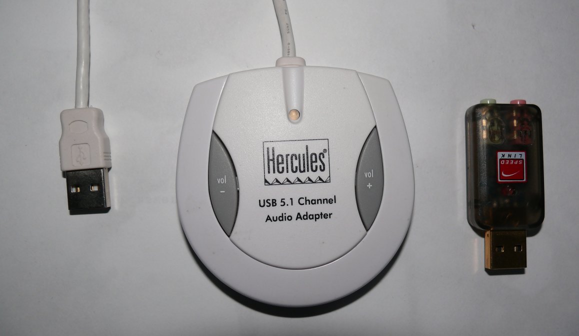
Use a line output, not a headphone output. The standard asks for 2 Hz to 10 kHz and a source impedance of 500 ohms or less. Headphone outputs roll off at the low end — the useful floor is nearer 20 Hz — and the association considered this enough of a problem to publish a dedicated amplifier for CD-player earphone outputs. The low-frequency content is not decorative: it carries the slow, large-area brightness variation across a frame.

Turn every enhancement off. Equalisation, loudness compensation, spatial or surround processing, automatic level control, noise suppression, “audio enhancements” of any description — each of them alters the waveform in ways designed for ears. On a modern desktop operating system these can be enabled by default. Anything that touches the samples between the encoder and the connector is a distortion of the picture.

Pin the sample rate. If the encoder generates 44.1 kHz and the system resamples to 48 kHz, the resampler’s filtering acts on the sync edges. Set the output device to 44.1 kHz, 16-bit, stereo, and confirm it rather than assuming.

Fix the output level and write it down. The output volume control directly scales the video amplitude that reaches the kit’s input, and the kit’s own R7 preset (Vol 2) is set against whatever level it was given. Changing the system volume after setting R7 de-tunes the whole chain. A repeatable, documented setting is worth more than a slightly better one.

Get the channel right. The standard puts video on the left channel and sound or separate sync on the right. On a 3.5 mm TRS plug, the tip is the left channel. A mono cable, or a cable wired to sum both channels, will mix whatever is on the right channel into the picture.

Bluetooth is not an option for the signal path. It applies lossy compression, for the reasons Vol 4 sets out. A wired connection is the only reliable one.

5.5 Sync Trim and Level Setting in Practice

Getting a picture is one thing; getting a stable one is a matter of three adjustments interacting, and the order to approach them in matters.

First, amplitude. The kit’s R7 preset scales the incoming signal to what the sync separator expects. Too low and sync separation is unreliable, the loop cannot hold, and the picture rolls or fails to lock at all. Too high and the picture clips — highlights flatten into featureless white. Set it with a signal known to be correct (Vol 4), not with home-made material.

Second, framing. If the picture locks but sits wrongly in the window, that is the taped sync hole’s position, not an electrical fault. Move the tape (Vol 2). The club’s own guide is explicit that horizontal placement is adjusted by moving the blanked hole.

Third, black level. Because the signal is AC-coupled, the black level floats with mean picture brightness. Where a black-level adjustment exists it is a refinement to be set last, once lock and framing are stable, and it is scene-dependent by nature.

An oscilloscope makes all three trivial and their absence makes all three guesswork. The single most valuable trace is the one described in Vol 2: the sensor’s pulse train with one pulse missing per revolution. The club’s fault-finding guide gives the signature precisely — a regular stream of pulses with a missing pulse every thirty-one.

5.6 Writing an Encoder: What the Builder’s Own Code Needs to Do

Software written for this kit belongs in this project’s code/software/ directory, with its own README carrying the build and run steps — not in these volumes, which hold the reasoning rather than the implementation. What follows is the specification such a program has to satisfy, gathered in one place.

For each frame, emit 3,528 samples at 44.1 kHz, 16-bit, on the left channel. Within the frame, produce 32 lines. Each line begins with a sync pulse of 4 to 11 samples at a level 33–50% below black, followed by active video whose amplitude tracks the brightness of that line of the picture, with white the more positive and the full black-to-white excursion spanning 1 volt peak to peak at the output. Omit the sync pulse between line 32 and line 1 and hold that interval at black. Order the lines so that line 1 is at the right-hand edge of the picture and line 32 at the left, and sample each line from the bottom of the picture to the top. Keep all content within 2 Hz to 10 kHz — which, given the resolution ceiling of roughly 50 elements per line, means resampling the source rather than letting sharp edges generate content above the band.

Three design notes beyond the specification:

• Generate a test pattern before generating a picture. A static grey ramp or a simple geometric pattern, produced by the same code path, makes every framing, ordering and polarity error immediately visible. A photograph or a webcam frame does not.
• Make polarity a runtime flag, not a compile-time decision. Vol 4 explains why the correct answer depends on the playback chain rather than on the format.
• Make it possible to write a wave file as well as stream. The same encoder that drives the kit live should be able to produce a file, because a file can be inspected in an audio editor, played on a different machine, and compared against the association’s own demonstration wave file sample by sample. That comparison is the fastest way to find an ordering error.

5.7 Cross-References

• The lock behaviour that makes buffer continuity the binding constraint: Vol 2.
• Every signal parameter an encoder must satisfy, with its source: Vol 3.
• Converting existing clips rather than generating signal, and the polarity tick-box: Vol 4.
• A published build that solved exactly this live-generation problem for a video game: Vol 6.
• The open questions this volume leaves — the unopened nbtv-design-tools archive among them: Vol 8.